EUT800 Digital Ultrasonic Flaw Detector

第 1 章 Preface 5

1.% 2statement 5

2.% 2Safety 5

3.% 2功能 Features 5

4.% 2index 6

5.% 2Promise 7

第 2 Chapter Using the Instrument 8

1.% 2仪器 Overview 8

1.1.% 3instrument 各 Part name 8

1.2.% 3operating 键 Disk description keyboard 布 Reasonable ，常 Located near by key 左 Thumb up 方位。Left hand maintain Just place it naturally 方 Convenient Adjust all settings of the instrument 置。8

1.3.% 3power supply 使用 9

1.3.1.% 4 Powered by AC power supply equipment 9

1.3.2.% 4 working on battery 10

2.1.4 Probe 连接 10

% 1.2仪器 operating 10

2.1.% 3instrument 基 This step 10

2.2.% 3start up 仪器 11

2.3.% 3screen 显 Show instructions 11

2.3.1.% 4 Function display item 11

2.3.2.% 4 Description of other indicators 12

2.4.% 3Features 概述 12

2.5.% 3Basic 操 Method of operation 13

2.5.1.% 4 Function Operation Example 13

第 3 章 Function Description 及 Operation method 14

1.% 2基本 Group function adjustment 14

1.1.% 3probe 范围 14

1.2.% 3material 声速 14

1.3.% 3pulse 移位 15

1.4.% 3Artifact 厚度 15

% 1.2探头 Group function adjustment 15

2.1.% 3Probe 方式 /Detection location 15

2.2.% 3refraction 角度 /Probe K 值 16

2.3.% 3Probe 前沿 /Probe zero 16

2.4.% 3Artifact 直径 /Scale method 17

% 1.% 2通道 Group function adjustment 17

3.1.% 3flaw detection 通道 17

3.2.% 3aisle 复制 18

3.3.% 3Set up 保存 /Settings modification 18

3.4.% 3Set up 删除 18

% 1.% 2存储 Group function adjustment 19

3.4.1 Group No 19

3.4.2 Call out 19

Chapter 1 Preface

Thank you for using our products. It is our great honor to be our customer. It is an intelligent digital ultrasonic flaw detector introduced by our company. It adopts the most advanced digital integration technology and new EL display technology. Its performance indicators have reached or exceeded the domestic advanced level, and it is also in the forefront in the world. The instrument uses artificial intelligence technology, which is powerful and easy to use. In order to enable you to grasp the operation process as soon as possible, we have provided a detailed operation manual. Please be sure to read this manual and other materials provided with the machine carefully before using the machine, which will help you to become familiar with it.

1.% 2 statement

Due to copyright, no part of this operation manual can be reproduced or used in any other way without our written permission. We are not responsible for damage caused by illegal use of the information contained in this operation manual. The company reserves the right to change the characteristics and contents of this operation manual without soliciting comments or prior notice.

2.% 2 safety

Do not use the instrument in heavy dust, humidity, strong magnetic fields, oil or corrosive environments. It is forbidden to wipe the case with soluble substances.

Use the power source provided by our company to charge the instrument.

When the instrument is not working for a long time, it should be charged and discharged regularly. It is recommended to do it once a month.

When connecting with external equipment (printer, PC), it must be done after turning off the power of the instrument. Do not disassemble or install the instrument without permission. In the event of repair, please contact the dealer or the company.

The instrument should be stored in a dry and clean place to avoid strong shaking.

3.% 2 Features

• Measurement display mode: A-type display mode;

• With linear suppression function, the maximum suppression is 80% of the screen height;

• Can switch between single crystal probe, dual crystal probe and two kinds of flaw detection working modes;

• With gate setting and alarm function. The position and width of the gate can be arbitrarily set on the screen, and the incoming wave alarm can be set;

• It has 500 independent inspection channels, and each channel has its own set of inspection parameters and DAC curve.

• With two display modes of angle and K value;

• DAC curve is automatically generated, up to 10 points can be recorded, and four additional adjustable offset curves;

• AVG curve is automatically generated, and two types of defects can be customized;

• Probe automatic calibration function;

• With storage function, it can store 100 A-scan graphs, parameters and DAC curves;

• Playback function of stored graphics, remove the stored A-scan graphics from the storage area and display on the screen

• With delete function, delete the specified content (represented by the storage group number) from the storage area;

• With peak memory function;

• Freeze and thaw function of waveform and flaw detection parameters;

• With sound path measurement and echo frequency analysis functions;

• With real-time power status indication function;

• Support wireless communication;

• Able to communicate with the PC, upload measurement data and system setting parameters to the PC for further processing (such as generating flaw detection reports, printing, etc.);

• The function of the instrument can be upgraded by using PC-side communication software;

• Lithium battery, low power consumption, continuous working for ten hours.

• Buzzer sound can be set during operation;

• Lightweight, convenient, and easy to operate.

4.% 2 indicator

Various performance indicators and technical parameters are shown in the following table:

name	Technical data
Scanning range (mm)	Scanning range (mm): 0 ～ 10000 Grades: 2.5, 5, 10, 20, 30, 40, 50, 60, 70, 80, 90, 100, 150, 200, 250, 300, 350, 400, 450, 500,600,700,800,900,1000,2000,3000,4000,5000,6000,7000,8000,9000,10000. Adjustment step: 1mm
Pulse shift (s)	Pulse shift (s): -20 ～ + 3400 Levels: -20, -10, 0.0, 10, 20, 50, 100, 150, 200, 250, 300, 350, 400, 450, 500, 600, 700,800,900,1000,1500,2000,2500,3000,3400. Adjustment step: 0.1 (-20s to 999.9s), 1 (1000s to 3400s)
Probe zero (s)	Probe zero: 0.0-99.99 Adjustment step: 0.01
Material sound velocity (m / s)	Material sound velocity: 1000 ～ 15000 7 fixed sound speeds: 2260, 2730, 3080, 3230, 4700, 5900, 6300 Adjustment step: 1
Way of working	Single probe (receiving and transmitting), dual probe (receiving and transmitting)
Frequency range (MHz)	Broadband 0.5–20
Gain adjustment (dB)	0 ～ 130 Adjustment step: 1, 2, 6, 12
Linear suppression	0% ～ 80% of screen height, step: 1%
Vertical linear error	Vertical linear error is not greater than 3%
Horizontal linear error	Within the scanning range, not more than 0.2%
Flaw detection margin	60dB
Dynamic Range	32dB
Call the police	Incoming wave alarm
Display	Display: High-brightness color flat panel display
A-Scan display area	Full screen or partial A-Scan display freezes and thaws A-Scan fills
Flaw detection channel	500
data storage	100 A-Scan graphics
Communication interface standard with PC	USB

Units of measurement	Mm
Power Adapter	Input 100V ～ 240V / 50Hz ～ 60Hz Output 9V / 1.5A
battery	Lithium battery 5000mAh
Working temperature (℃)	-10 ～ 50
Operating humidity (RH)	20% ～ 90%
Interface Type	BNC
Overall dimensions (mm)	238 × 160 × 48
Weight (kg)	1.0

5.% 2 Convention

In order to facilitate the use of this manual, all the operating steps, precautions, etc. are arranged in the same way. This helps to find each piece of information quickly. The directory structure of the manual goes to the fourth level of the directory. Items below the fourth level are shown in bold headings.

Attention and instruction sign

Note: Attention signs indicate characteristics and special aspects that may affect the accuracy of the results during operation. Note: A note can include a special introduction to other chapters or a feature.

Item list

The list of items is represented by the following form item A

Item B

…

Chapter 2 Using the Instrument

1.% 2 Instrument Overview

1.1.% 3 Name of each part of the instrument

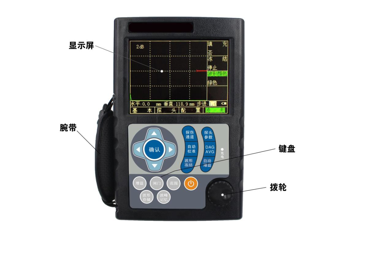
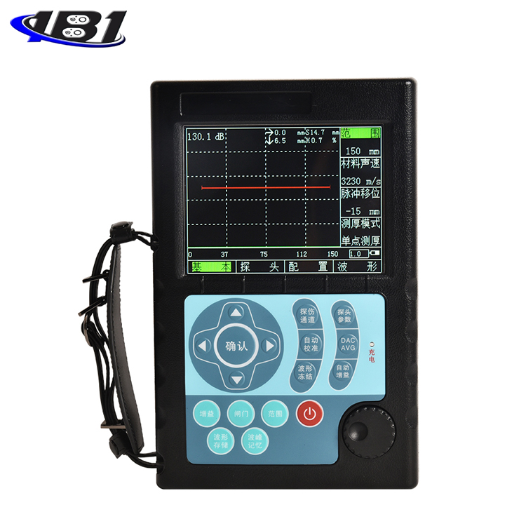
Figure 2.1 Appearance of the instrument

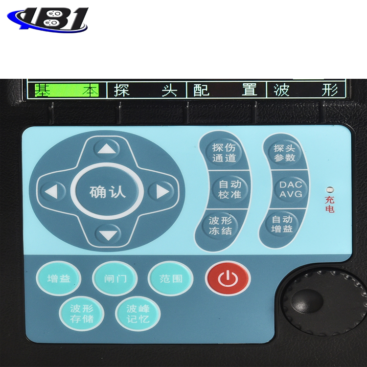
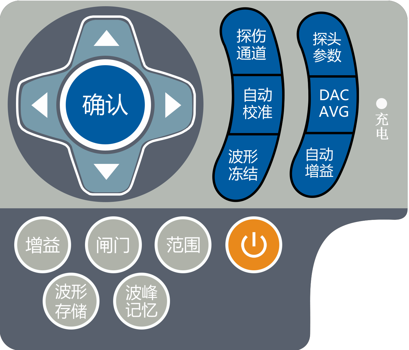
1.2.% 3 Operation keyboard description The keyboard layout is reasonable, and the commonly used keys are located near the thumb of the left hand. You can easily adjust all the settings of the instrument by keeping the left hand in a natural state.

In order to facilitate the operator to identify the functional characteristics of the keyboard, all keys are grouped and marked with different colors according to their operating characteristics. The key area on the left is frequently used keys. The right key area is a shortcut menu key, which is used to quickly switch to the menu of the corresponding function, and also reflects the operation process of the instrument. The lower left area is a shortcut function key for quickly implementing common functions.

The keyboard layout is shown below:

Operation procedure of this instrument:

Figure 2.2 Keyboard layout

Select flaw detection channel-> select probe type-> auto-calibrate probe and other parameters-> make curve (DAC, AVG, AWS)

——> Stored in the channel ——> Site flaw detection

(Auto gain and peak memory are the most commonly used function keys in the typical operation process above, so they are placed in this area.) For detailed operation instructions of the keys, see Appendix II \"\" Operation List \".

1.3.% 3 Power usage

It can be operated using a plug-in power supply (AC.DC adapter) or battery.

When using the power adapter as the working power source, the instrument will automatically detect and switch to the adapter power after plugging in the power adapter. When the battery is used as the working power source, the instrument will automatically detect and switch to battery power when the power adapter is disconnected.

With the battery installed, the battery can be charged when connected to the power adapter's power supply system.

1.3.1.% 4 Powered by AC power supply equipment

Connect to AC power via a dedicated AC adapter.

Do not forcibly unplug the power supply during the operation of the instrument, because at this time, if the battery power is low, the instrument will automatically power off and cannot be shut down normally. The correct method is to turn off the instrument and then unplug it.

1.3.2.% 4 working with battery

When using battery power, use our recommended battery products.

The battery box is on the back of the instrument. Use a screwdriver to open the battery compartment cover. Put the battery in the battery compartment. Insert the plug of the battery into the socket of the battery.

There is a battery level symbol above the waveform display area, as shown below:

Battery level is low. Battery level is low. Figure 2.3 Battery level display

If the symbol of low battery power appears, you should immediately stop the inspection, replace the battery or recharge.

Note: If you need to perform on-site measurements, please bring a spare battery with you.

Charge the Li battery

Lithium batteries can be charged using an external battery charger. It is recommended to use the power adapter in the standard case of the instrument for charging. Before using this charger, please read its instructions carefully. The continuous charging time of a lithium (4Ah) battery is approximately 4-5 hours. The charge indicator turns off when charging is complete.

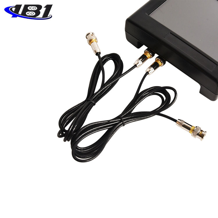
1.4.% 3 Probe connection

When using the test, you need to connect the appropriate probe. As long as there is a proper cable and the operating frequency is within the appropriate range, any probe produced by our company is suitable. The probe connector is BNC.

The probe is connected to the socket above the instrument housing. In the single-probe mode, only the transmit jack is valid. The connection of the dual crystal link can be freely connected.

% 1.2 Instrument operation

2.1.% 3 Basic operation steps of the instrument

% 4) Prepare the workpiece to be tested;

% 4) Insert the probe cable plug into the socket above the main unit and tighten the plug;

% 4) Press 2.1.3 to select a working power supply, click , and turn on;

% 4) Program loading and power-on self-test;

% 4) Under normal circumstances when powering on, it automatically enters the state when it was last powered off. The instrument parameters are the same as when the power was last turned off, but the waveforms when the power was last turned off are not displayed. When the power-on self-test is abnormal, you can shut down and then restart. If the self-test still fails, you can force reset to the state when the instrument leaves the factory.

% 4) Check the battery voltage. If the battery power detection icon is shown in Figure 2.3, if the battery power is insufficient;

% 4) Do you need to calibrate the instrument and draw DAC or AVG curve? If necessary, professional technicians will perform related operations (see Chapter 4);

% 4) Call up the parameter setting of the corresponding flaw detection channel;

% 4) measurement;

% 4) store the data to be saved;

% 4) shut down;

2.2.% 3 Start the instrument

Press the , the screen will start after the startup tone and enter the program loading process. The whole loading process takes about 4-5 seconds. After the program is loaded, the system performs a self-test and enters the operation interface.

2.3.% 3 Screen display instructions

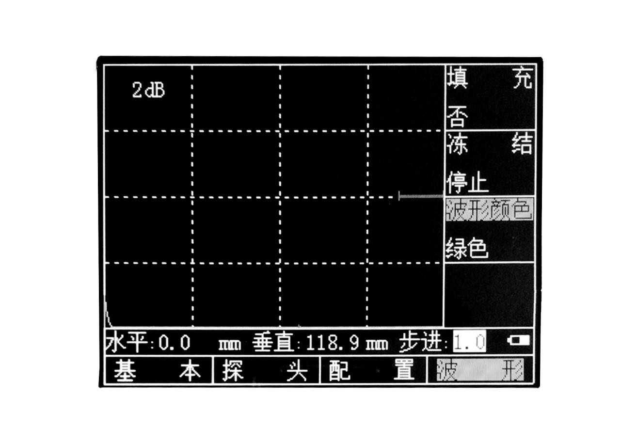
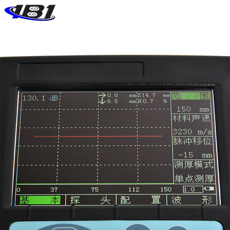
Figure 2.4 Screen Description

The interface is divided into the right menu and the lower menu. In the interface, H is the value of the wave height inside the gate, and S is the sound path value of the wound trapped by the gate. . The upper left corner of the menu is the current gain value of the instrument. The horizontal and vertical in the interface are for oblique probes. When the oblique probe calibration is completed, the instrument will automatically calculate the vertical depth and horizontal distance of the wound wave relative to the probe according to the probe angle. The step in the interface is the minimum range for changing the instrument parameters each time. Changing the step can quickly get the desired parameters.

1.% 2.% 3.% 4 Function display items

The names of the sixteen function groups are displayed on four pages at the bottom of the screen. The currently selected function group is highlighted. At the same time, the currently selected function menu in the current function group is also highlighted. The currently selected function menu and parameters appear above the graphic display area.

2.% 2.% 3.% 4 Other instructions

In addition to the status bar data and symbols showing some settings, readings, and status indicators, above the function menu are highlighted measurement values and some status indications of the current operation. There are freeze and communication signs next to the battery level indicator.

Sign	name	meaning
S	Interval value flag	Distance of sound path from the point of incidence to the point of reflection.
H	Waveform value flag	The wave height value from the incident point to the reflection point.

% 1.% 2.5 Feature Overview

The function implementation is divided into sixteen menu-type function groups and several special functions.

16 menu-type function groups are distributed in 4 function pages, including basic (BASE), probe (PROBE), channel (CHAN), memory (MEM), gate (GATE), self-calibration, DAC1, DAC2, AVG1, AVG2 , TX, Gain, B-scan, Setting 1, Setting 2, The functions of each AWS functional group are described in the table below.

页	Functional group	Features	description
1	Basic	Detection range, material sound velocity, pulse shift, material thickness	Display required basic parameters Reconciliation
1	Probe parameters	Probe angle / K value, probe leading edge, scale delay / dual	Probe related settings
1	Configuration	Buzzer, AWS, Suppression, Repeat Frequency	Auxiliary correlation
1	Waveform	Fill, freeze, waveform color, B-scan
2	Gate 1	Gate A start, Gate A width, Gate A height	Gate setting related items
2	Gate 2	Gate A start, Gate A width, Gate A height	Gate setting related items
2	Auxiliary function	Open hotspot, connect software, language, auto wave height	Accessibility related
2	Self-calibration	Straight probe calibration, (left button) oblique probe calibration,	Automatic probe calibration
2	DAC	Curve on, set point, calibration gate, curve mode	DAC curve calibration
3	DAC configuration	DAC waste line / DAC quantitative line, DAC evaluation line, flaw detection standard	DAC curve settings
3	AVG	Curve open, reference type, calibration gate	AVG curve calibration
3	AVG configuration	Curve equivalent, probe frequency, wafer diameter, equivalent display	AVG curve settings
3	aisle	Flaw detection channel, save, delete, initialize	Items related to flaw detection channel
4	storage	Group number, recall, save, delete	Data storage settings
4	Oblique probe calibration	Calibration On, Probe Delay, Probe Angle, Calibration Gate
4	Straight probe calibration	Calibration on, workpiece thickness, calibration gate
4	Waveform recording	Video group number, whether to open, whether to record, whether to delete
	Gain	Compensation gain, add gain, scan gain \ auto gain, surface compensation	Gain related settings

Other special functions can be realized through special function keys. The functions of the special function keys are described in the table below.

special function	Function description
freeze	Waveform freeze

Peak memory	Keep curve maximum on each pixel line along the horizontal direction of the screen
Measured value display	Select how measured values are displayed on the screen
confirm	Alternate function menu switching, parameter coarse and fine adjustment switching, function confirmation, etc.

% 1.% 2.6 Basic operation method

The function group selection can be completed by ; the selection of a specific function menu can be completed by Up and Down keys; at this time, the parameters of this function menu can be changed by . In addition, some function menus are multiplexed with two functions. When a function has been selected, press (turn the knob down) to switch to another function.

Coarse and fine-tuned functions

Some functions can be selected between coarse and fine adjustment. When switching to the corresponding function, press(knob down) again to switch between these two adjustment modes. Fine-tuning is identified by \"* \" in front of the function item.

The following functions can be selected for coarse and fine adjustment.

Function group

Detection range is basic

Material sound velocity basic

Pulse shift basic

Basic workpiece thickness

6.1.% 3.% 4 Example of function operation

Assume that the detection range function adjustment in the basic function group is currently selected. If you want to select the gate logic of the gate function group, how to operate? First select the gate function group via the shortcut key; then press the up and down keys to select the gate logic / gate alarm function menu. As the function menu is the gate

The gate logic and the gate alarm are multiplexed, so if the gate logic is displayed at this time, the operation is completed; if the gate alarm is displayed, press the key (

Button pressed) to the gate logic. After the selection is completed, you can use the to adjust the gate logic.

When the function option to be selected is not on the same page as the currently selected function, you can use to switch the function page.

Chapter 3 Functional Description and Operation

1.% 2 Basic group function adjustment

In the basic function group, you can adjust the function items related to the setting display range, including the detection range, material sound speed, pulse shift, and workpiece thickness. During the flaw detection process, the range displayed on the screen is related to the material of the workpiece and the properties of the probe. Workpiece material affects the propagation rate of ultrasonic waves

degree.

1.1.% 3 Detection range

Set the measurement range displayed on the screen during testing, that is, the size of the observation window. Range: 0mm ～ 10000mm or 0.1\"～ 400\"

If the detection range function menu is currently selected, you can switch between coarse adjustment and fine adjustment by pressing the .

Coarse adjustment: 2.5mm, 5mm, 10mm, 20mm, 30mm, 40mm, 50mm, 60mm, 70mm, 80mm, 90mm, 100mm,

150mm, 200mm, 250mm, 300mm, 350mm, 400mm, 450mm, 500mm, 600mm, 700mm, 800mm,

900mm, 1000mm, 2000mm, 3000mm, 4000mm, 5000mm, 6000mm, 7000mm, 8000mm, 9000mm,

10000mm

Fine-tuning: range step

≤100.0mm0.1mm

> 100mm1.0mm

operating:

• Use to select the detection range function menu, and then use to adjust the detection range parameter, that is, the interval value.

• Use the to switch between coarse and fine adjustment methods.

1.2.% 3 material sound velocity

You can set the rate at which ultrasonic waves travel through the workpiece. Range: 1000m / s ～ 9999m / s or

If the material sound speed function menu is currently selected, you can switch between coarse adjustment and fine adjustment by pressing the . Coarse adjustment: 2260m / s copper medium transverse wave sound velocity

Longitudinal sound velocity in 2730m / s plexiglass

3080m / s Aluminum Transverse Wave Sound Velocity

Sound velocity in the transverse wave of 3230m / s steel

4700m / s copper longitudinal wave sound velocity

5900m / s steel longitudinal wave sound velocity

6300m / s Aluminum mid-longitudinal sound velocity Fine adjustment: Step length is 1m / s or

operating:

• Select the basic function group with , and select the material sound speed function menu with the up and down keys, and then use the to adjust the sound speed parameters.

• Use the to switch between coarse and fine adjustment methods.

Note: Be sure to ensure the accuracy of the sound velocity value. Some measurement results displayed on the instrument status line are calculated based on this sound velocity value.

1.3.% 3 pulse shift

You can set the pulse shift during the flaw detection process, that is, the D delay. Changing the D delay can adjust the starting position of the waveform. In this way, the starting point of the display pulse can be adjusted so that it is located on the surface of the workpiece or a starting surface inside the workpiece. If the pulse must start from the surface of the workpiece under test, the D delay must be set to zero.

Range: -15µs to 3400µs Step size: 1µs

operating:

• Use the switch function page.

• Select the basic function group with , and select the pulse shift function menu with the up and down keys, and then use the to adjust the pulse shift parameter, which is the D delay value.

1.4.% 3 Workpiece thickness

Set the thickness of the workpiece to be tested during flaw detection. Workpiece thickness: 1mm ～ 1000mm

If the thickness function menu is currently selected, you can switch between coarse adjustment and fine adjustment by pressing the .

Coarse adjustment: 1mm, 5 mm, 10 mm, 20 mm, 50mm, 100mm, 200mm, 300mm, 400mm, 500mm, 600mm,

700mm,

800mm, 900mm, 1000mm

Fine adjustment: <100 mm0.1mm

> 100 mm1.0mm

operating:

• Use the switch function page.

• Select the basic function group with , select the workpiece thickness function menu with the up and down keys, and then use the to adjust the workpiece thickness. Use to switch between coarse and fine adjustment methods.

% 1.2 Probe group function adjustment

This function group can adjust and set the functions related to ultrasonic transmission and reception, probe mode / detection position, refraction angle / probe K value, probe zero / probe front, scale method / workpiece diameter. The inherent nature of the probe determines the probe zero.

Note: In order to accurately set the speed of sound and the zero point of the probe in the workpiece, please refer to Chapter 4 \"Calibration of the Instrument\".

2.1.% 3 Probe method / detection position

Probe method:

If the probe used is a single probe, it is set to a straight probe, an oblique probe; if it is a dual-crystal probe, it is set to double; if it is a penetrating probe, it is set to transmission. Options: straight probe, oblique probe, dual crystal, transmission

operating:

• Use the switch function page.

• Select the probe function group with , select the probe mode function menu with the up and down keys, and use the to set the probe mode.

• When the probe method is selected. The corresponding default probe settings are loaded. Parameters such as sound speed, detection range, gain, angle, probe zero, and leading edge are all given typical values.

Detection location:

Set the detection position of the probe when detecting flaws in a circular tube.

Options: Outer circle: The probe is located on the outer wall of the round tube. At this time, the corrected d value represents the depth of the defect from the outer wall surface, and the L value represents the distance of the defect from the front edge of the probe along the outer wall surface;

Inner wall: The probe is located on the inner wall of the round tube. At this time, the corrected d value represents the depth of the defect from the inner wall surface, and the L value represents the distance of the defect from the probe's front edge along the outer wall surface.

operating:

• Use the switch function page.

• Select the probe function group with , select the function menu of detection position with up and down keys, and then adjust the detection position with .

• Use the to switch the detection position and workpiece diameter functions.

2.2.% 3 refraction angle / probe K value

When measuring with an oblique probe, in order to calculate the position of the reflector, the probe refraction angle needs to be entered correctly in advance. Since some probes have a nominal value that is not an angle value, but a K value, a K value entry for the probe is added for convenience . The refraction angle and the K value of the probe are the same parameter. Changing one of the values will change the other. The relationship between the two is: the K value of the probe = the tangent of the refraction angle.

Refraction angle: Step: 0.1 Operation:

• Use the switch function page.

• Use the function keys to select the probe function group, use the up and down keys to select the refraction angle function menu, and then use the to adjust the refraction angle.

• Use the to switch the refraction angle and probe K value function. Probe K value:

Step size: 0.1

operating:

• Use the switch function page.

• Use the to select the function group of the oblique probe, use the up and down keys to select the function menu of the probe K value, and then use the to adjust the probe K value.

• Use the to switch the refraction angle and probe K value function.

2.3.% 3 Probe leading edge / probe zero

Probe front:

Set the leading edge of the probe, which is the point of incidence of the sound beam. Range: 0.00mm to 50.0mm

Step length: 0.01mm

operating:

• Use the switch function page.

• Select the probe function group with , use the up and down keys to select the probe front function menu, and then use the to adjust the probe front.

• Use to switch the function of probe front and scale mode.

Probe zero:

You can set the probe zero during the flaw detection process, which is the P delay. The P delay must be used to compensate the probe's delay due to the sound path from the transducer to the workpiece under test.

Range: 0µs to 99.99µs

Step size: 0.01µs

• Use the switch function page.

• Select the probe function group with , and then select the probe zero function menu with the up and down keys, and then use the to adjust the probe zero parameter, which is the P delay value.

Note: If P delay is unknown, please refer to Chapter 4 Instrument Calibration.

2.4.% 3 Workpiece diameter / scale method

Workpiece diameter:

Range: 5.0mm ～ 5000mm

Step length: <100 mm0.1mm

> 100 mm1.0mm

operating:

• Use the switch function page.

• Select the probe function group with , select the workpiece diameter function menu with the up and down keys, and adjust the workpiece diameter with the dial.

• Use the to switch the detection position and workpiece diameter functions.

Scale method:

The scaling method refers to the definition method of the horizontal coordinates of the screen curve display area, including four methods: \"Sound \", \"Projection \", \"Depth \", and \"Surface \". This function is effective when the refraction angle input value is not zero. When the refraction angle is zero, the coordinate is defined as the sound path mode.

Options: sound path, depth operation:

• Use the switch function page.

• Select the probe function group with , select the scaling mode function menu with the up and down keys, and then use the to select the scaling mode.

• Use to switch the function of probe front and scale mode.

% 1.% 2 Channel group function adjustment

The channel function group is used for channel-related operations, including flaw detection channels, channel copying, setting saving / setting modification, and setting deletion.

3.1.% 3 Flaw detection channel

Due to the need to inspect a variety of workpieces during field inspection, or to change the probe during the inspection process, the instrument needs to be recalibrated in these cases. For the convenience of instrument adjustment, the instrument provides 500 inspection channels. Users You can adjust the settings needed for various scenes in advance and store them in different channels, and you can directly switch to the corresponding channels to recall these settings during the scene.

Range: No.1 ～ No.500 Operation:

• Use the switch function page.

• Select the channel function group with , select the function menu of the flaw detection channel with the up and down keys, and then adjust the sequence number of the flaw detection channel with the .

• During the process of automatically turning the flaw detection channel, the data in the flaw detection channel will be automatically loaded, and the stored channel will be loaded to the stored instrument.

Settings, empty channels will load the initial settings.

3.2.% 3 Channel Copy

The function of copying the parameters of the flaw detection channel is implemented. After the copy is successful, the flaw detection parameters of the current channel will be copied to the target channel. operating:

• Use the switch function page.

• Use the function keys to select the channel function group, use the up and down keys to select the channel copy function menu, and then use the to adjust the target channel number.

• After setting the target channel number, if you press the key at this time, the channel copy will be performed.

Note: When the target channel already has data or the current channel has no stored setting parameters, executing the channel copy function will prompt an operation error.

3.3.% 3 Setting saving / setting modification

Setting saving: The function menu saves the detection channel settings. operating:

• Use the switch function page.

• Select the channel function group with , and then use the corresponding menu key to select the setting to save the function menu, and then use the to perform the storage operation.

Note: 1. If * is displayed in front of the channel number of the inspection channel, it means that the channel has the setting value.

% 1. If there are already setting parameters in this channel, the setting save operation will update the original setting value.

% 1. If the current channel is locked, the setting save function is invalid.

% 1. If the channel data cannot be deleted due to a program error, the function \"Init \" option is deleted, but this function will delete the storage settings of all channels, so it is recommended to use it only when necessary.

Setting modification: To realize the function of rewriting the setting parameters of the flaw detection channel where the data has been stored. After successful execution, the current machine settings will replace the flaw detection parameters stored in the current channel.

operating:

• Use the switch function page.

• Use the function key to select the channel function group, use the up and down keys to select the setting and modify the function menu, and then use the to perform the recall operation.

• If there is no setting parameter for the current channel, this function menu always shows off when adjusting with the ; if there is setting parameter for the current channel, a\"Yes / No\" prompt will be displayed when adjusting with the . If you press , the extraction will be executed. If you press any other key, the call will be canceled.

3.4.% 3 delete settings

This function menu deletes the detection channel settings. operating:

• Use the switch function page.

• Select the channel function group with , and then select the setting and delete function menu with the corresponding menu key of the function menu, and then use the to delete the function.

• If there is no setting parameter for the current channel, this function menu always shows off when adjusting with ; if the current channel has setting parameters and the channel

If it is not locked, the prompt\"\" Yes / No\"\" will be displayed when adjusting with the . At this time, if you press the , the deletion will be executed. If you press any other key, the deletion will be cancelled.

% 1.% 2 Storage group function adjustment

It is used to adjust the storage mode, recall, delete, save and other related functions of setting data and flaw detection parameters. Including data group number, data recall, data save, data delete function menu.

Note: When the waveform is stored, the stored data includes the current A-scan waveform data and the current flaw detection parameters and DAC curve of the instrument. This

It means that when extracting a set of stored data, not only the currently displayed waveform will change to the stored waveform, but also the current instrument detection parameters will also change to the stored parameters.

4.1.% 3 Group number

Set the storage group number.

Range: waveform storage, group number 1 ~ 500

operating:

• Use the switch function page.

• Select the storage function group with , select the group number function menu with the up and down keys, and set the group number with the .

• Use the to switch the storage mode.

Note: In the waveform storage mode, if * is displayed before the group number, it indicates that the group has data; if ￥ is displayed before the group number, it indicates that the group has data and is locked;

4.2.% 3 Recall

Realize the data recall function in the waveform storage mode. Extract the data corresponding to the current group number. After successful recall, the current waveform and flaw detection parameters will be replaced by the stored waveform and flaw detection parameters, and the waveform will be frozen.

operating:

• Use the switch function page.

• Use to select the storage function group, use the up and down keys to select the function menu, and then use the or to perform the recall operation.

• If there is no data in the current group number, this function menu always shows off when adjusting with the ; if there is data in the current group, the prompt\"\ Yes / No \" will be displayed when adjusting with the . Press to execute the extraction. If you press any other key, it will be called to cancel.

4.3.% 3 Storage

This function menu implements data storage. operating:

• Use the switch function page.

• Use the to select the storage function group, use the up and down keys to select the save function menu, and then use the orto perform the storage operation.

• You can also use the storage shortcut to directly implement the storage operation. The data will be automatically stored in the first empty space from the first group.

Note: 1. Before storing data, you must ensure that there is no data in the data group corresponding to the current group number, otherwise it is invalid.

% 1. The current storage mode is set correctly.

% 1. If you need to upload the waveform screen with DAC curve to the PC, you should first adjust the settings and DAC parameters, and then store the data under this group number.

4.4.% 3 delete

Data deletion. Delete the data corresponding to the current group number. \"* \" Before the group number disappears after the deletion is successful. operating:

• Use the switch function page.

• Use the to select the storage function group, use the up and down keys to select the delete function menu, and then use theto perform the delete operation.

% 1.% 2 Gate group function adjustment

Regarding the adjustment of gate setting related items. Including gate logic, gate alarm, gate start, gate width, gate height. The role of the gate in flaw detection:

• Monitor the workpiece for defects within the set logic and range, and if so, alarm.

• Measure the position and size of defect echoes.

With double gate function: Gate A and Gate B. Generally, only the gate A can be used to monitor the workpiece defects; the double gate is mainly used for the measurement and calibration of multiple echoes, such as measuring the distance between the surface of the workpiece and the primary echo during thickness measurement.

5.1.% 3 Gate logic / gate alarm

This function menu has gate alarm reuse. When this function menu is selected, you can switch the function by pressing . operating:

• Use the switch function page.

• Select the gate function group with shortcut keys, use the up and down keys to select the gate logic function menu, and then use the to adjust the gate logic.

• Use to switch gate logic and gate alarm functions. Gate alarm:

Gate alarm setting.

According to the setting of the gate logic, it can be used for incoming wave alarm. That is, when the echo amplitude is higher than the gate threshold, the buzzer will alarm. operating:

• Use the switch function page.

• Select the gate function group with the shortcut key, use the up and down keys to select the gate alarm function menu, and then use the to switch the alarm function on and off.

• Use to switch the gate alarm function.

5.2.% 3 Gate A start / B gate start

The function menu A gate start and B gate start are multiplexed. When this function menu is selected, you can switch the function by pressing the .

A Gate start: Operation:

• Use the switch function page.

• Use the shortcut keys to select the gate function group, use the up and down keys to select the A gate starting function menu, and then use the to adjust the gate A starting position.

• Use to switch the A and B gate start functions.

B Gate start: Operation:

• Use the switch function page.

• Use the shortcut keys to select the gate function group, use the up and down keys to select the gate B function menu, and then use the to adjust the gate B start position.

• Use to switch the A and B gate start functions.

Note: Gate B and Gate A are independent of each other. The gate start, gate width, and gate height can be adjusted independently without interference.

5.3.% 3 Gate width A / B gate width

The function menu A gate width, B gate width are reused. When this function menu is selected, the function can be switched by pressing the .

A Gate width: Operation:

• Use the switch function page.

• Select the gate function group with shortcut keys, use the up and down keys to select the function menu for gate A, and then use the to adjust the width of gate A.

• Use to switch the gate width function of A and B.

B Gate width: Operation:

• Use the switch function page.

• Use the shortcut keys to select the gate function group, use the up and down keys to select the gate B function menu, and then use the to adjust the width of gate B.

• Use to switch the gate width function of A and B.

5.4.% 3 Gate A / B Gate Height

The function menu A gate threshold and B gate threshold are reused. When this function menu is selected, the function can be switched by pressing the .

A Gate height:

Set the height of gate A. The parameter is expressed as a percentage, which is a percentage relative to the full amplitude. Range: 2% to 90%

operating:

• Use the switch function page.

• Use the shortcut keys to select the gate function group, use the up and down keys to select the A gate height function menu, and then use the to adjust the gate A height value.

• Use to switch between A and B altitude functions.

B Gate height:

Set the height of gate B. The parameter is expressed as a percentage, which is a percentage relative to the full amplitude. Range: 2% to 90%

operating:

• Use the switch function page.

• Use the shortcut keys to select the gate function group, use the up and down keys to select the B gate height function menu, and then use the to adjust the gate B height value.

• Use to switch between A and B altitude functions.

% 1.% 2 Probe self-calibration function adjustment

6.1.% 3 Straight Probe Calibration

In order to facilitate the operator to calibrate the zero point of the straight probe and the sound velocity of the material, the instrument provides a probe calibration function, which can be used to conveniently complete the straight probe calibration. The straight probe calibration function is located in the self-calibration function menu.

Take the standard straight probe as an example, it is a single crystal probe with a frequency of 2.5MHz and a diameter of 20mm. Calibration requires two test blocks of the same material and thickness as the measurement object.

Assuming that the probe is calibrated with a test block with a thickness of 100mm, the steps are as follows: First set an approximate sound velocity value such as 5920m / s

Step 1: Select (Automatic Calibration Button) Select Straight Probe Calibration-Turn on the automatic calibration function (Display: Whether it is valid Adjust to (Yes) Step 2: Set the thickness of the workpiece (higher than known thickness)

Step 3: The probe is connected, coated with couplant, placed on the workpiece to be tested, and found the echo

Step 4: Adjust to the calibration gate (cover the echo with the gate-click on the automatic gain, and the echo height will reach 80% of the screen). In the (calibration gate column, click to confirm the key) so that the straight probe calibration is completed.

Note: Auto calibration can also be used on a single test block of known thickness. Operators can use multiple echoes without having to separate probes

Put on the thick test block and thin test block, move the gate A to each echo and input the correct thickness value.

6.2.% 3 Calibration of oblique probe

In order to facilitate the operator to calibrate the oblique probe angle, leading edge, zero point and material sound speed, the instrument provides the oblique probe calibration function. Using this function can conveniently complete the calibration of the oblique probe. The tilt probe calibration function is located in the self-calibration function menu. For automatic calibration of oblique probes, this instrument provides two methods. The first method is based on the CSK-1A test block calibration.

1. Calibration based on CSK-1A test block (one-button automatic calibration method (Enter key))

Taking the standard oblique probe as an example, it is a single crystal probe with a frequency of 2.5MHz, a chip of 13mm × 13mm and an angle of K2. It can be calibrated using the CSK-IA test block. No parameters need to be entered before calibration.

Step 1: Select (Auto Calibration Button) to select the oblique probe calibration-turn on the automatic calibration function (display: whether it is effectively adjusted to (Yes) Step 2: Connect the probe front end to the semi-circle direction, the flaw detector will automatically adjust the gate to double Gate, automatic placement of gate position, automatic setting

Set the detection range. Place the probe on the center of the circle and move it back and forth to find the highest wave of R100. At the same time, ensure that the wave of R50 is higher than 15%. Press the confirmation key twice.

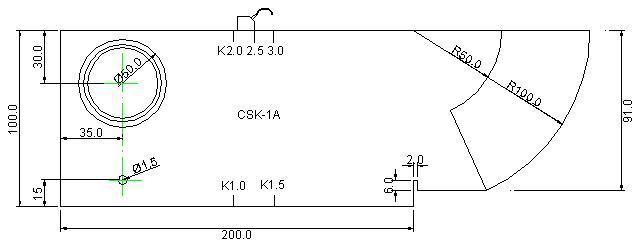
200.0

Figure 3.1 CSK-IA test block

3) Press the Enter key again to display the estimated value of the probe's leading edge. This value needs to be read out from the probe to the center of the scale (or measured with a scale), and then input using the dial.

Step 3: Align the probe with the direction of the circle of the transparent glass, find the highest wave at the place marked K2, cover the waveform with the gate, and calibrate the probe angle according to the confirmation

The entire calibration process does not need to manually adjust the detection range and gate, just find the highest wave and press Enter to confirm.

Figure 3.2 Angle measurement

6.3.% 3 Gate A / A Gate Width

The function menu A gate start and A gate width are reused. The reset of A gate start and A gate width here is to facilitate the adjustment of the gate parameters during probe calibration. When this function menu is selected, please refer to 3.5 for the adjustment method .2 and 3.5.3.

6.4.% 3 Calibration type

CSK-IA.

% 1.% 2 DAC1 group function adjustment

The DAC function group is used to calibrate the DAC curve. Including DAC curve switch / calibration correction switch, DAC calibration point / DAC correction point, A gate start / A gate width, display calibration / curve mode.

For the DAC curve, please refer to 4.4:

7.1.% 3 DAC curve / calibration correction

The function menu DAC curve display switch and calibration correction switch are multiplexed.

DAC curve:

Realize the DAC display switch function. If the DAC is turned on, the DAC curve is displayed. The DAC curve switch is invalid. Options: On, Off

operating:

• Use the switch function page.

• Select the DAC1 function group with the DAC shortcut key, select the DAC curve function menu with the up and down keys, and use the to set the DAC

Curve switch.

• Use to switch DAC curve and calibration correction functions.

Note: When more than 3 calibration points are completed, the DAC curve is automatically drawn. You can set up to 10 calibration points.

Calibration correction:

Recalibrate the correction points selected in 3.7.2. If, when making a DAC curve, you find that a calibration point previously calibrated is not ideal due to large calibration errors or calibration errors, you can select the corresponding calibration point and adjust the gate to the corresponding position, and re-calibrate through the calibration correction function Calibrate the data at that point.

Options: On and off operations:

• Use the switch function page.

• Select the DAC1 function group with the DAC shortcut key, use the up and down keys to select the calibration correction function menu, and then use the to correct the calibration point.

• Use to switch DAC curve and calibration correction functions.

7.2.% 3 DAC calibration / correction point

The function menu DAC calibration point and correction point selection function are reused. When this function menu is selected, you can switch the function by pressing the key.

can.

The DAC calibration point function menu is used to record the echo information needed to make a DAC curve. The correction point selection function is used to select the correction that needs to be performed.

Calibration point.

DAC calibration point: Range: 3 ~ 10 Operation:

• Confirm that the gate is working in a single gate state.

• Use the switch function page.

• Select the DAC function group with the DAC shortcut key, and select the DAC calibration point function menu with the up and down keys.

• Make the reference echo fall inside the gate, then adjust to (calibrate the gate) and press the confirmation key-to add the calibration point. Repeat the same operation to continue adding the calibration point.

• Use to switch between DAC calibration point and correction point selection. Range: 1 ~ 30, but not greater than the value of the DAC calibration point

Note: When the calibration point is wrong-you can re-calibrate by turning on the curve again.

7.3.% 3 Gate A / A Gate Width

The function menu A gate start and A gate width are multiplexed. The reset of A gate start and A gate width here is for the convenience of DAC.

Adjust the gate parameters when calibrating the point. When this function menu is selected, please refer to the description in 3.3.2 and 3.3.3 for the adjustment method. operating:

• Select the DAC function group with the DAC shortcut key, use the up and down keys to select and display the calibration function menu, and use the to switch the display function of the calibration point.

• Use to switch between display calibration and curve mode functions. Curve mode:

The curve mode is used to select the connection method between the DAC calibration points. Options: line, curve

operating:

• Use the switch function page.

• Through the DAC shortcut key DAC function group, use the up and down keys to select the curve mode function menu, and use the to select the DAC curve connection mode.

• Use to switch between display calibration and curve mode functions.

% 1.% 2 DAC2 group function adjustment

The DAC2 function group is used to adjust the relevant parameters required for setting the DAC curve. Including DAC waste line / equivalent standard, DAC quantitative line,

DAC evaluation line, DAC bus.

In order to adapt to the drawing standards of DAC curves in different industries, the instrument provides 3 DAC curves with adjustable offset, which are DAC waste line, DAC quantitative line, and DAC evaluation line. In addition, in order to adapt the DAC curve to different environmental conditions, a gain compensation function is also provided. The offset values of the three offset curves are relative to the bus bar. The bus bar is drawn using the data information of the calibration points and the attenuation law of the ultrasonic wave during the propagation process. The order of evaluation is distributed on the screen from top to bottom.

8.1.% 3 DAC waste line / equivalent standard

The function menu DAC waste line and equivalent standard selection function are reused. When this function menu is selected, you can switch the function by pressing the .

DAC waste line:

Set the offset value of the DAC waste line.

Parameter range: -50dB ～ 50dB with 1 dB step

operating:

• Use the switch function page.

• Select the DAC2 function group with , select the DAC waste line function menu with the up and down keys, and use the to set the offset value of the DAC waste line.

• Use the to switch between DAC waste line determination and equivalent standard selection. Equivalent standard:

The equivalent standard refers to which curve the defect echo equivalent value is based on, which is commonly used as \"bus\" or \"quantitative\". The bus refers to the original calibration curve of the DAC. The other three optional standards are the DAC offset curve. This standard only takes effect after a successful DAC curve has been made.

Options: bus, discard, quantify, evaluate operation:

• Use the switch function page.

• Select the DAC2 function group with the , select the equivalent standard function menu with the up and down keys, and use the to select the reference curve for calculating the equivalent.

• Use the to switch between DAC waste line determination and equivalent standard selection.

8.2.% 3 DAC line

Set the offset value of the DAC line.

Parameter range: -50dB ～ 50dB with 1 dB step

operating:

• Use the switch function page.

• Select the DAC2 function group with , select the DAC fixed line function menu with the Up and Down keys, and set the DAC with the

Quantitative curve offset.

8.3.% 3 DAC evaluation line

This function menu is used to adjust the evaluation line in the DAC offset curve. Parameter range: -50dB to 50dB with a step size of 0.1 dB

operating:

• Use the switch function page.

• Select the DAC2 function group with , select the DAC evaluation line function menu with the Up and Down keys, and use theto set the DAC

Evaluate the offset of the curve.

8.4.% 3 Flaw detection standard

The flaw detector has 14 built-in flaw detection standards, \"Custom, GB / T 11345-89A, GB / T 11345-89B, GB / T 11345-89C, JB / T 4730-2005, JG / T 3034.1 / 2, SY / T 4109-2005, GB / T 3559-94, ASME-3, DL-T 820-2002 A, DL-T 820-2002

B, DL-T 820-2002 C, TB 10212-98D (butt weld), TB 10212-98J (corner weld) \". Among them Custom is customizable

Typical curve, others are fixed standards. Under this option, press the Enter key to enter the standard setting interface. You can set the workpiece thickness and the test block. Some standards automatically adjust the curve offset according to these two parameters.

operating:

• Use the switch function page.

• Select the DAC2 function group with the , select the standard function menu of the flaw detection with the up and down keys, and set the standard offset value of the echo curve with the dial.

% 1.% 2 AVG1 group function adjustment

With AVG curve measurement function, the AVG1 function group is used to set AVG curve calibration parameters. Includes AVG curve switch, probe name, probe frequency / chip size, reference type / reference size.

9.1.% 3 AVG mode

This function menu is AVG mode and wedge sound speed multiplexing. When this function menu is selected, you can switch the function by pressing .

AVG mode:

Implement the AVG display switch function. If AVG is turned on, the AVG curve will be displayed. Options: On and off operations:

• Use the switch function page.

• Select the AVG function group with the AVG shortcut key, use the up and down keys to select the AVG mode function menu, and use the to set the AVG.

Curve switch.

• Select the AVG1 function group with the AVG shortcut key, select the wedge sound speed function menu with the up and down keys, and use the to switch the AVG

mode.

9.2.% 3 Probe frequency / chip size

(AVG curve configuration) The probe frequency and chip size of this function menu are reused. When this function menu is selected, the probe frequency:

Enter the nominal frequency of the probe used.

Range: 0.5MHz ~ 10MHz Operation:

• Use the switch function page.

• Select the AVG function group with the AVG shortcut key, use the up and down keys to select the probe frequency function menu, and then use the to adjust the probe frequency.

• Use the to switch between probe frequency and chip size functions. Wafer size:

Nominal effective diameter of the probe. Range: 3.00mm ～ 35.00mm

• Use the switch function page.

• Select the AVG1 function group with the AVG shortcut key, use the up and down keys to select the wafer size function menu, and then use the to adjust the wafer size.

• Use the to switch between probe frequency and chip size functions.

9.3.% 3 reference type / reference size

The function menu has the same reference type and reference size. When the function menu is selected, you can switch the function by pressing the key. Reference type:

When calibrating AVG curves, a standard test block with a known regular reflector is required. The AVG curve calibrated by this instrument supports three types of regular reflectors.

Options: Flat-bottomed hole: a cylindrical hole whose diameter on the bottom surface is comparable to the size of the reference defect. Large flat bottom: The reflector size can be approximated as an infinite plane.

operating:

• Select the AVG1 function group with the AVG shortcut key, use the up and down keys to select the reference type function menu, and then use the to adjust the type of the reference reflector.

• Use to switch between reference type and reference size. Reference Size:

The nominal size of a regular reflector on a standard test block. Range: 0.50mm ～ 10.0mm

operating:

• Use the switch function page.

• Use the function keys to select the AVG function group, use the up and down keys to select the reference size function menu, and then use the to adjust the nominal value of the reflector.

• Use to switch between reference type and reference size.Gate A / AVG curve

A Gate start:

The reset of the A gate start here is for the convenience of AVG calibration to adjust the gate position. When this function menu is selected, please refer to the description in 3.3.2 for the adjustment method.

AVG curve:

The AVG curve is calibrated based on the known reflector on the standard test block. When the reference reflector specified in the standard does not match the size of the reflector on the test block, the AVG curve can be adjusted to its equivalent curve.

Range: 0.30mm ～ 20.0mm Operation:

Select the AVG2 function group with , select the AVG curve function menu with the up and down keys, and then use the to adjust the AVG curve equivalent value.

• Use to switch the function of A gate start and AVG curve.

9.4.% 3 Calibration reference

This function is used to calibrate the AVG curve.

Options: 0 (uncalibrated), 1 (calibrated) Operation:

• Confirm that the gate is working in a single gate state.

• Use the switch function page.

• Select the AVG configuration function group with , and select the calibration reference function menu with the up and down keys.

• Move gate A to the desired reference echo and let the reference echo fall inside the gate.

• Gain the echo in gate A to 80% of the screen.

• Use the right button to calibrate the AVG curve reference value.

• If you need to modify this reference value, you can delete it with the left button and recalibrate.

9.5.% 3 Transmission repetition frequency

In order to generate ultrasonic waves, the number of pulses that the probe chip is excited by a pulse generator per second is called (ultrasonic emission) repetition frequency. This parameter is used to set the ultrasonic transmission repetition frequency (PRF) of the instrument system.

Adjustment range: (30 ~ 1000) Hz, general setting (100 ~ 300) Hz is appropriate. When the speed of the flaw detection and scanning of the workpiece is fast, a higher repetition frequency needs to be selected to prevent the defect from being missed. When the scanning speed is slow, setting a lower emission repetition frequency can reduce the power consumption of the instrument.

If the detection range is large, such as greater than 2000mm, it is recommended not to transmit more than 100Hz. Can adjust the pulse frequency of the flaw detector

% 1.% 2 Gain group function adjustment

The gain function group is used to adjust the system sensitivity, making the gain adjustment flexible and convenient. Includes automatic gain.

10.1.% 3 automatic gain

The automatic gain function is a tool for quickly adjusting the instrument's gain (dB). It can automatically adjust the instrument's gain value so that the echo peak value captured in the A gate reaches the set screen height (such as 80%). Setting range (10% to 100%)

operating:

• Use the switch function page.

• Select the gain function group with , select the auto gain function menu with the up and down keys, and turn the to adjust the set height.

10.2.% 3 Dynamic playback / video recording

Recording: This function enables real-time waveform recording and reporting on the host computer.

10.3.% 3 video group number / delete

This function menu is used to adjust the group number of the current flaw detection video.

Note: This function enables real-time waveform recording and reporting on the host computer.

% 1.% 2 Set 1 group function adjustment

The instrument's detection method / echo suppression, coordinate grid / ELD brightness settings are all implemented in this group.

11.1.% 3 detection method / echo suppression

Detection method:

Select the measurement method. When the measurement method is peak mode, the measurement value is the echo data with the highest amplitude in the gate. In the edge measurement mode, the measurement data is the intersection of the leading edge of the echo (the rising line of the echo waveform curve) and the gate. Therefore, when the edge mode is selected, the measurement value of the echo amplitude in the gate is affected by the gate threshold (height).

Options: peak, edge operation:

• Use the switch function page.

• Use the shortcut key to select the setting 1 function group, use the up and down keys to select the detection mode function menu, and then use the to set the measurement mode.

• Use to switch the detection mode and serial port setting function. Echo suppression:

This function menu is used to suppress the echo display amplitude, for example, to remove the structural noise of the measured workpiece. It is to suppress the display of echoes whose amplitude is lower than the set value by setting the suppression percentage (ie, the percentage of full amplitude).

The percentage of suppression (ie, the percentage of full amplitude) indicates the smallest displayed echo height. The amplitude of echoes below this height will be ignored and recorded as zero amplitude.

Range: 0% ~ 80% Step: 1%

operating:

• Use the shortcut key to select the setting 1 function group, use the up and down keys to select the echo suppression function menu, and then use the to set the suppression percentage.

Note: Please use this function with caution, so as not to suppress the injury wave while suppressing the noise. In addition, this feature is disabled in some flaw detection specifications.

% 1.% 2 Setting function adjustment

12.1.% 3 color selection

Selection of color:

The instrument screen has four different color configuration schemes. Operators can choose the appropriate interface according to their own habits and operating environment. Options: 0 to 4

operating:

• Use the switch function page.

• Use the shortcut key to select the setting 2 function group, and use the up and down keys to select the color selection function menu. Then use the to select the appropriate color scheme.

Use to switch the software version and color selection function.

12.2.% 3 WIFI to PC

After entering this mode, you can connect to a PC to upload flaw detection data.

% 1.% 2 Special function adjustment

In order to facilitate user use, in addition to the menu-type function group selection on the instrument panel, there are thirteen special function keys with high frequency of use, including gain step adjustment, gain +/-, waveform freeze, peak memory, dynamic recording, measurement Value display, detection range, pulse shift, gate A, gate

13.1.% 3 Gain step size

Adjust the gain step.

Options: 1.0dB, 2.0dB, 6.0dB ,,,, 100.0dB

operating:

• Press the , the gain step will cycle through the options.

13.2.% 3 gain value

When the gain step is adjusted to a suitable option, then the gain size can be set by the gain + / gain-keys. Parameter range: 0dB ~ 130dB

operating:

• Press the or key, and the gain will change with the currently set gain step.

13.3.% 3 freeze

Achieve waveform freeze function.

operating:

• Press to switch the waveform between frozen and unfrozen.

• In the frozen state, a reminder icon * appears on the screen.

Note: In the frozen state, some function adjustments are disabled.

13.4.% 3 peak memory

The function of the peak memory function is to capture and memorize the peak points of the echo on each pixel line of the abscissa when the probe is moved on the test block, and connect them to form an envelope. According to the shape of the envelope, the user can conveniently Find the highest wave of the defect, and can provide a basis for judging the nature of the defect.

operating

• Press to switch the peak memory switch.

• When the peak memory function is on, a prompt appears on the screen。

13.5.% 3 Flaw Detection Video

Press this button to start or stop the recording of the flaw detection process automatically.

13.6.% 3 measured value display

A measurement data is displayed in the upper right corner of the graphic display area. This function is to select the content of the displayed data. When one of the data of sound path, projection activity or depth is displayed here, the other two data will be displayed in the status bar. When the equivalent dB is selected to be displayed, the screen will display the equivalent value and sound measured by the DAC curve. If the DAC curve is closed or the waveform in the gate exceeds the screen height range, the equivalent dB will be displayed as *.

Options: sound path, projection, depth, equivalent dB, equivalent hole operation

• Press to sequentially switch the type of displayed data.

13.7.% 3 Shortcut Function Key

The detection range, gate A, and gate B are high-frequency functions, so shortcut keys are set. operating

• Press to quickly switch the function menu to the A gate starting option. If you continue to press this key, the function menu will switch between A gate starting, A gate width, and A gate height.

13.8.% 3 Restore factory settings

If necessary, you can initialize the instrument in the flaw detection channel menu bar.Chapter 4 Calibration and Measurement of the Instrument

1.% 2 DAC curve application method

The DAC curve is used to distinguish changes in the amplitude of reflectors of the same size but at different distances. Under normal circumstances, the reflectors of the same size and different distances within the test specimen will cause changes in the amplitude of the wave due to the attenuation of the material and the spread of the beam. The DAC curve is graphically compensated for material attenuation, near-field effects, beam spread, and surface finish. Under normal circumstances, after the DAC curve is drawn, regardless of the position of the reflector in the test piece, the echo peaks generated by the reflector of the same size are on the same curve. For the same reason, the echoes generated by the smaller reflectors than the reflectors will fall below the curve, while the larger ones will fall above the curve.

1. Select the detection channel Select the channel function group via the shortcut key, adjust the detection channel number, and select a channel as the instrument setting channel under the current detection conditions, for example: No.1. (Note: A set of DAC curve calibration points can be saved under each channel. These calibration points do not need to be saved. When the calibration points are calibrated, they will be saved directly under the current channel. If you want to save the current instrument simultaneously under this channel, For parameter setting, you need to complete the operation through \"\" Channel \"->\" Setting Save \".)

2. Turn on the DAC curve function, select the DAC1 function group with the shortcut key, and then use the up and down keys to select the DAC curve function menu (if there is no DAC curve function in the current submenu, please use the to switch the DAC curve and calibration correction functions). Then press to set the DAC curve switch.

3. Make DAC curve Select the DAC1 function group by shortcut key and add calibration points as described in 3.7.2 of this manual. After adding two calibration points, the DAC curve will be automatically drawn on the screen of the instrument. (Note: Please calibrate the data from small to large along the detection range, that is, the post-calibration point should be behind the previous calibration point, and its echo height should not be higher than the previous calibration point. The point DAC curve is drawn as a straight line.)

4. Adjust the offset values of the three offset curves. Select the DAC2 function group through the shortcut key, and adjust the offsets of the three offset curves according to the detection standard, that is, adjust the offset of the DAC evaluation line, DAC quantitative line, and DAC waste line. Value to the required setting.

5. The drawn DAC curve is shown in the figure:

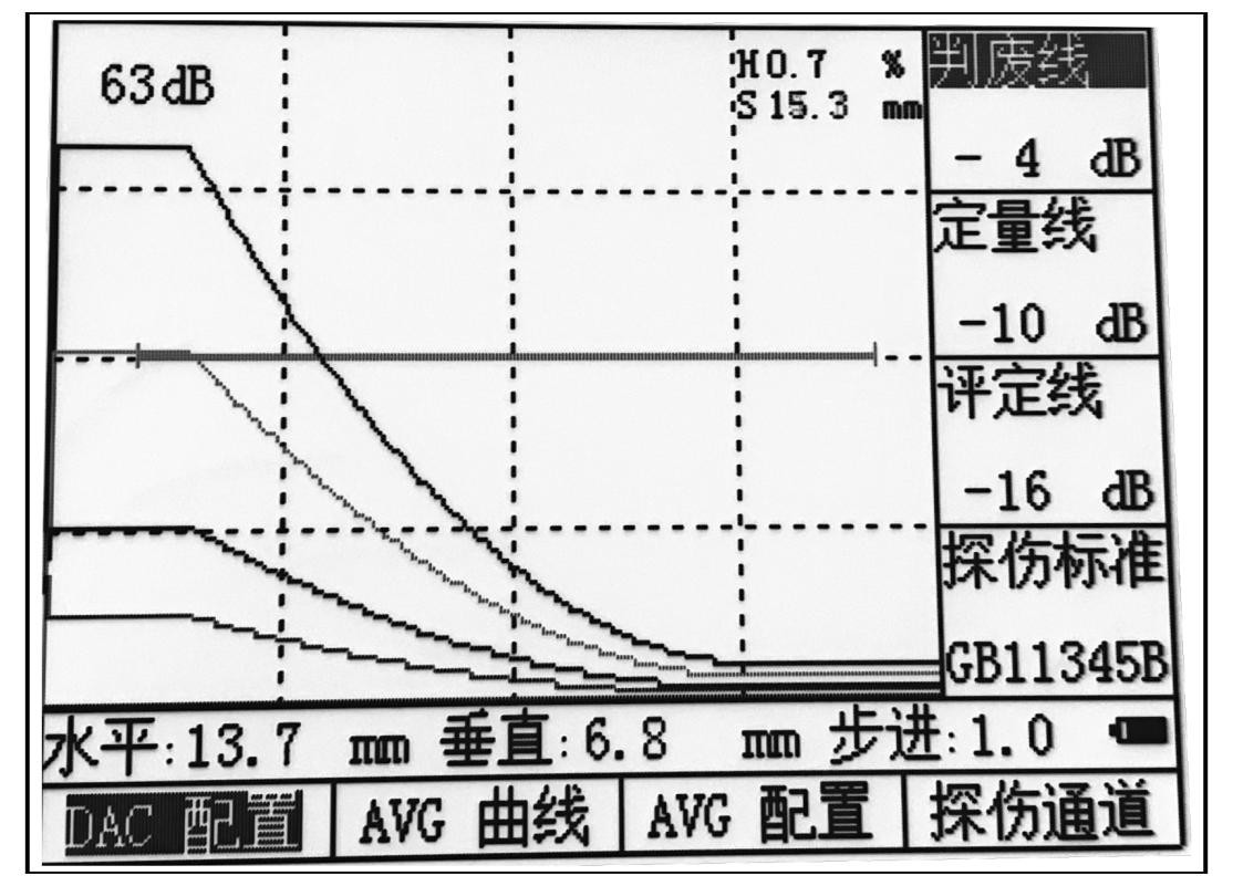
Figure 4.4 DAC curve

As shown in the figure above, the three DAC curves divide the screen into three areas: I, II, and III. These three DAC curves will be drawn on the screen during on-site inspection. The operator can directly determine the defect according to the area where the echo height of the reflector is located. nature.

7. Equivalent calculation If you want to measure the equivalent value of the defect echo in the gate, you can use the to select the measured value display function, switch the displayed value in the upper right corner of the screen to the equivalent value, and then select DAC1 through the shortcut key. Function group, use the up and down keys to select the equivalent standard function, adjust the equivalent standard and use the corresponding DAC offset curve as the measurement standard.

2.% 2 measurement content

The measurement using this flaw detector requires the following work:

Set the gate starting point, gate width, gate threshold and gate alarm mode. The measurement content is:

S sound path

Relative value of echo height in H (%) gate range (relative to screen height)

absolute value of echo height in h gate range (unit is pixel)

d defect depth

D (%) Relative value of defect depth (relative to workpiece thickness)

The horizontal distance between the P defect and the probe's leading edge

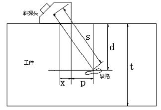
among them:

s: represents the sound path;

d: the depth of the defect;

t: the thickness of the workpiece;

x: the distance from the ultrasound source to the leading edge of the probe;

p: indicates the horizontal distance of the defect from the front of the probe;

D: is the relative value of the defect depth, it is obtained according to the following method

D  d t

When a straight probe is used, the x, p, d, and D values are meaningless because the d and S values coincide. The x value does not need to be set, and the p, d, and D values will not be displayed.

Before taking measurements:

The calibration of the instrument including the speed of sound and the zero point of the probe should be completed. The measured amplitude is the echo amplitude with the highest amplitude in the gate. In the leading edge measurement mode, the measured sound path is the sound path value at the leading edge of the echo (the rising line of the echo waveform curve). Therefore, when the leading edge method is selected, the measurement value of the echo amplitude in the gate is affected by the gate threshold (height).

Sound path measurement can only be measured when the gate is open. Before measurement, first select the measurement method: edge mode, peak mode. Then select single and double gates. In the single gate mode, the measured value is the sound path value at the foreword or peak of the echo in the gate. In double-gate mode: the measured value is the sound path value between the echo in gate A and the echo in gate B.

Chapter 5 Maintenance and Repair

1.% 2 environmental requirements

Strictly avoid collisions, heavy dust, humidity, strong magnetic fields, and oil pollution. It is forbidden to wipe the case with soluble substances.

2.% 2 battery charge

The battery status indicator on the display screen reflects the battery voltage situation in real time. When the battery voltage is too low, the battery status indicator on the screen is the undervoltage indicatorThe instrument should be charged as soon as possible.

The charging method is as follows (both on and off):

% 3. Insert the power plug of the power adapter into the charging socket;

% 3. Connect the power adapter to 220V / 50Hz city power, the charging indicator is on;

% 3. When the charge indicator is off, the battery is fully charged. Under normal conditions, it can be fully charged after about 4.5 hours of charging.

% 3. Unplug the charging plug and the charging process is finished.

Tips: 1. The input voltage of the power adapter is 220V AC and the output is 9V DC. The maximum charging current is about 1000mA and the longest charging time.

About 6h.

% 1. This instrument uses a lithium-ion battery, so when the under-voltage mark appears, it should be charged in time. Over-discharge will damage the battery.

% 1. If the instrument is not used for a long time, please recharge the instrument every other month to prevent the battery from being used normally due to over-discharge.

% 1. If the battery cannot be charged normally due to over-discharge (the battery is empty and the charging indicator is off), you can unplug the power adapter two minutes later and then plug it in to continue charging. Repeat this operation multiple times to charge the battery Back to normal.

% 1. The instrument can work while charging.

3.% 2 Troubleshooting

If the instrument has the following abnormal conditions:

% 3. The instrument cannot be turned off automatically;

% 3. Cannot measure;

% 3. The keys do not work;

% 3. The measured value is erratic.

% 3. Please do not disassemble the machine for self-repair. After completing the warranty card, please send the instrument to our company's maintenance department to implement the warranty regulations. If you can briefly describe the error situation and send it together, we will thank you very much.

4.% 2 safety tips

The instrument is designed to meet the relevant safety standards. In use, it must meet the specified external environmental conditions, and the operator must have a corresponding technical background to ensure safe operation. Before putting the instrument into use, please read the following safety tips carefully:

Note: 1. This instrument is a non-destructive testing instrument for material testing and is not allowed to be used as a medical instrument.

2. This instrument is limited to use in laboratory and industrial environments.

System power

The instrument can be powered either by an external power adapter or by a lithium-ion battery. When selecting the power adapter and battery, please use our recommended products.

For battery charging and battery replacement, please follow our operation steps.

system software

No software can avoid errors, but we strive to minimize the chance of such errors. The software of this instrument has been thoroughly and rigorously tested.

Unexpected failure

When the following abnormal conditions occur, it indicates that the instrument has failed. Please turn off the power of the instrument and remove the battery if necessary. Take the instrument to the designated service station for repair.

% 3. The instrument suffered significant mechanical damage (such as severe crushing or collision during transportation);

% 3. Instrument keyboard or screen display is abnormal;

% 3. Long time storage in high temperature, high humidity or corrosive environment;

appendix

Appendix I Notice to users

I. After the user purchases our products, please fill out the\"Warranty Registration Card\" carefully and affix the official seal of the user unit. Please send a copy of the (1) Lianhe purchase invoice to the customer service department of the company, or you can entrust the sales unit to send it on behalf of the customer. (2) Sending (reserving) the local branch maintenance station for registration. If there is no maintenance station, please send (1) and (2) to the customer service department of our company. When the procedure is incomplete, it can only be repaired without warranty. Second, the company's products from the date of purchase, quality failure within one year (except non-guaranteed parts), please \"warranty card\" (user retention coupon) or a copy of the purchase invoice with the company's branches Contact a repair station to repair the product, replace or return it. During the warranty period, you cannot show the warranty card or a copy of the purchase invoice. The company calculates the warranty period based on the factory date, and the period is one year.

Third, the company's products beyond the warranty period of failure, maintenance stations in various places are responsible for after-sales service, product maintenance, according to the company's regulations to check the maintenance fee. 4.\"Special configuration\" (special-shaped probes, special software, etc.) outside the company's stereotyped products will be charged according to relevant standards.

5. Any damage caused by the user to disassemble the company's products, damage to the product due to improper transportation, storage or incorrect operation according to the \"Product Instruction Manual \", as well as altering the warranty card without permission, the company cannot guarantee .

Appendix II Operation List

The operation of the instrument is realized by directly triggering the keys on the panel or a combination of several keys. The table below gives the specific illustration of the keys on the operation panel, and the names and functions of the keys.

Icon	name	Function Description	chapter
	Arrow keys	In menu mode, the left and right keys are used to select the function group, and the up and down keys are used to adjust the function group. Function item selection. In full screen mode, the left and right keys are used to move the gate, and the up and down keys are used to increase or decrease the gain.	3.1 ～ 3.15
	Shuttle button	You can rotate and adjust the parameters and change the content of the options. Press this knob for the function	3.1 ～ 3.15
	Gain	Press the gain key, the cursor will shift to the position of the gain value, and then use the dial to adjust the gain. Press the gain key again, the cursor will shift to the gain step position, and then use the dial to adjust the gain step. The gain adjustment range is 0dB ~ 120dB. Gain step size is 0dB, 0.1dB, 0.5dB, 1dB, 2dB, 6dB, 12dB.	3.17.2
	Gate	Press the gate key, the screen can quickly switch to the function menu of gate A, press this key to connect The function menu can be switched among the three functions of A gate start, A gate width, and A gate height, and the corresponding functions can be quickly adjusted.	3.17.9
	Automatic gain	The automatic gain function is a tool for quickly adjusting the instrument's gain (dB). It can automatically adjust the instrument's gain value so that the echo peak value captured in gate A reaches the set screen height, such as 80%. The setting range is from 10% to 100% 。	3.17.7
	Peak memory	Press the peak memory key to enable or disable the peak memory function.	3.17.6
	Soft power switch	Switch instrument	2.2.1

Appendix III. Examples of Weld Inspection

One. Preparation before flaw detection

Digital ultrasonic flaw detector

2. Transverse wave oblique probe: 5M13 × 13K2

3. Standard test blocks: CSK-IB, CSK-3A 4. Butt welding seam of 30mm thick steel plate

5． DAC parameters:

(1) DAC points: d = 5, 10, 15, 20 (mm) 4 points

(2) Offset of waste line: -4dB

(3) Quantitative line offset: -10dB

(4) Evaluation line offset: -16dB

6. Coupling agent (such as: motor oil, etc.) II. Selection of detection surface

Three on one side of the weld. Boot

1. Connect the probe to the ultrasonic flaw detector

2. Turn on the panel switch, start the self-test, and enter the flaw detection interface. four. calibration

1. Input material sound speed: 3230m / s

2. Probe leading edge calibration

(1) As shown in Figure 1, place the probe on position 0 of the CSK-1B standard test block

(2) Move the probe back and forth so that the echo amplitude of the arc surface of the test block R100 is the highest, and the echo amplitude should not exceed the screen, otherwise the gain needs to be reduced.

(3) When the echo amplitude reaches the highest level, keep the probe stationary and mark the side of the probe corresponding to the \"0 \" scale of the test block. This point is the incident point of the beam

(4) Front distance calibration:

Read the scale value corresponding to the \"0 \" scale of the test block directly from the probe scale, which is the leading edge value of the probe. (Or use a scale to measure the L value shown in Figure 1, with the leading edge x = 100-L.)

3． Calibration of probe zero

(Figure 1) Schematic diagram of zero point and leading edge of CSK-IA test block calibration

Place the probe as shown in Figure 1, cover the highest wave with the gate, and adjust the probe zero point until the sound path S = 100

4． Probe K value calibration (calibration of refraction angle)

Due to the material of the measured object and the wear of the wedge, the actual K value of the probe will have some errors with the nominal value. Therefore, the actual K of the probe needs to be determined

value. The calibration steps are as follows:

(1) Place the probe on the appropriate angle mark of the CSK-1A standard test block as shown in Figure 2.

(2) Move the probe back and forth to keep the probe still when the echo peak of the large circular hole on the side of the test block is found.

(3) On the test block, read the K value of the incident point aligned with the test block. This angle is the actual K value of the probe. Enter this value. (Or by calculating the slope calibration, when the menu focus is under the probe angle option, press thekey, the menu displays \"L = 80.0 \", you can actually measure the L value, use +,

-Press the key to enter the L value, then press again, the flaw detector will automatically calculate the K value, see figure 2 below)

35P

K = P + Xd =

50 °

60 °

70 °

(Figure 2: Calibration of refraction angle)

Fives. Making a DAC curve

Making DAC curve with CSK-3A test block

Step 1: Move the probe to find the hole depth as

The highest echo of 10mm, and cover the A gate with this wave, press \"+ \" key to increase the calibration point to \"1 \";

Step 2: Move the probe to find the hole depth as

The highest echo of 20mm, and cover the A gate with this wave, press \"+ \" key to increase the calibration point to \"2 \";

At this point, 2 calibration points have been added.

The DAC curve has been generated. According to the needs of flaw detection, you can continue to find the hole depth of 30,

The highest echoes of reflectors such as 40 and 50mm increase the calibration points to 3, 4, and 5. Step 3: Enter the criteria

On the DAC2 menu, set the judging line offset to -4dB, the quantitative line offset to -10dB, and the evaluation line offset to -16dB.

six. On-site inspection

1. By adjusting the flaw detection sensitivity, the DAC curve is completely displayed on the screen, and then the flaw detection is started.

2. When detecting flaws, generally make the probe run perpendicular to the weld and make a zigzag scan along the weld (ie the probe's movement track is the probe);

3． The distance the probe moves along the weld (forward and backward): 0 ~ 100mm (such as the following figure) Calculation method: Starting point (position 2): 0

End point (position 2): S = 2KT = 2 × 2 × 25 = 100mm (where K is the probe slope and T is the workpiece thickness)

4. The speed of the probe moving along the weld (left and right): ≤1.5 m / min

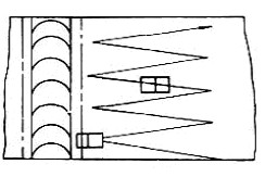
Seven. Store flaw detection waveform and data

Store the flaw detection waveform and data to the corresponding group number.

Eight. It will be connected with the computer, upload the testing waveform and data to the computer, and generate the testing report.

Appendix IV Terminology

This appendix lists the terms used in this manual for ultrasonic nondestructive testing. Knowing the exact meanings of these terms will help you better use this manual.

1. Pulse amplitude: The voltage amplitude of the pulse signal. When using type A display, it is usually the height from the baseline to the peak of the pulse.

2. Pulse length: The duration of the pulse as a time or period value.

3. Decibel: Logarithmic representation of two amplitude or intensity ratios.

4. Acoustic impedance: The ratio of the sound pressure of a sound wave to the velocity of a particle's vibration, usually expressed as the product of the density p and the velocity c of the medium.

5. Acoustic impedance matching: Coupling between two media with equivalent acoustic impedance.

6. Attenuation: When the ultrasonic wave propagates in the medium, the sound pressure gradually decreases as the propagation distance increases.

7. Total attenuation: The sound pressure of a particular waveform of any shape will increase with the propagation distance, and will decrease due to a combination of scattering, absorption, and sound beam diffusion.

8. Attenuation coefficient: When ultrasonic waves propagate in the medium, the loss of sound pressure within a unit distance due to material scattering is usually expressed in decibels per cm.

9. Defect: Size, shape, orientation, location or nature will cause damage to the effective use of the workpiece, or discontinuities that do not meet the requirements of the specified acceptance criteria.

10. Type A display: An information representation method that uses horizontal baseline (X axis) to indicate distance or time, and deflection perpendicular to the baseline (Y axis) to indicate amplitude.

11. Transmit pulse: An electrical pulse applied to a transducer in order to generate an ultrasonic wave.

12. Time Baseline: Horizontal scanning lines representing time or distance in a type A display phosphor screen.

13. Scan: Repeated movement of the electron beam across the flaw detector screen in the same pattern.

14. Scanning range: the maximum sound path that can be displayed on the baseline at the time of the phosphor screen.

15. Scanning speed: the ratio of the horizontal axis on the phosphor screen to the corresponding sound path.

16. Delayed Scanning: Scanning method in which the beginning of the baseline is not displayed in the A or B display.

17. Horizontal linearity: The signal displayed on the time or distance axis of the ultrasonic flaw detector screen and the signal input to the receiver (via a corrected time generator

Or multiple echoes from a plate of known thickness).

18. Vertical linearity: The degree to which the signal displayed on the time or distance axis of the ultrasonic flaw detector screen is proportional to the amplitude of the signal input to the receiver.

19. Dynamic range: The ratio of the maximum and minimum reflection area wave height that can be resolved on the screen of the ultrasonic flaw detector when the gain adjustment is unchanged. It is usually expressed in decibels.

20. Pulse repetition frequency: In order to generate ultrasonic waves, the number of pulses of the probe chip excited by a pulse generator per second.

21. Detection frequency: the frequency of ultrasonic waves used in ultrasonic testing. It is usually 0.4 MHz to 15MHz.

22. Echo frequency: the reciprocal of the peak interval time obtained by the echo on the time axis.

23. Sensitivity: A measure of the smallest ultrasonic signal that produces a discernible indication on the screen of an ultrasonic flaw detector.

24. Sensitivity margin: The difference between the standard defect detection sensitivity and the maximum detection sensitivity in a certain level in an ultrasonic flaw detection system.

25. Resolution: The ability of an ultrasonic flaw detection system to distinguish two adjacent defects of a certain size that are closest to each other in the transverse, longitudinal or depth direction.

26. Suppression: In ultrasonic flaw detectors, in order to reduce or eliminate low-amplitude signals (electrical or material noise), a control method to highlight larger signals.

27. Gate: An electronic method selected for monitoring a flaw detection signal or for further processing.

28. Attenuator: A device that changes the signal voltage (sound pressure) quantitatively. The amount of attenuation is expressed in decibels.

29. Signal-to-noise ratio: The ratio of the amplitude of the ultrasound signal to the amplitude of the maximum background noise. It is usually expressed in decibels.

30. Blocking: The phenomenon that the receiver's sensitivity is reduced or fails immediately after receiving the transmitted pulse or strong pulse signal.

31. Gain: The logarithmic form of the voltage amplification of the receiving amplifier of the ultrasonic flaw detector. Expressed in decibels.

32. Distance wave amplitude curve (DAC): A set of three parameters drawn from the distance of the known reflector, the gain of the flaw detector and the size of the reflector according to the specified conditions. In actual flaw detection, the measured defect distance and gain value can be used to estimate the defect equivalent size from this curve.

33. Coupling: It plays the role of conducting acoustic waves between the probe and the object under test.

34. Test block: a sample used to identify the characteristics and sensitivity of the ultrasonic testing system.

35. Standard test blocks: Test blocks whose materials, shapes and sizes have been verified by the competent authority or authoritative organization. It is used to test the performance and sensitivity of the ultrasonic testing device or system.

36. Contrast test block: a test block that adjusts the sensitivity of the ultrasonic inspection system or compares the size of the defect. Generally made of materials with similar characteristics to the material being tested.

37. Probe: An electroacoustic conversion device that transmits or receives (or both transmits and receives) ultrasonic energy. The device typically consists of a trademark, plug, housing, backing, piezoelectric element, protective film, or wedge.

38. Straight Probe: Probe for vertical flaw detection, mainly used for longitudinal wave flaw detection.

39. Oblique probe: Probe for oblique flaw detection, mainly used for transverse wave flaw detection.

Appendix V National and Industry Standards Related to Ultrasonic Flaw Detection

The national standards and industry standards for ultrasonic flaw detection involved in this manual are:

1.GB/T 12604.1-90 terms for non-destructive testing Ultrasonic testing

2.JB / T 10061-1999 A pulsed ultrasonic flaw detector general technical requirements

3. JJG 746-2004 Ultrasonic Flaw Detector National Metrological Verification Regulations of the People's Republic of China

Packing card

Serial number	name	Quantity	unit
1	Flaw detector host	1	台
2	Straight probe	1	只
3	Oblique probe	1	只
4	Power Adapter	1	个
5	BNC probe with cable	2	根
6	user's manual	1	本
7	Instrument case	1	个
8	Data processing software	1	套

Products

contact us

table of Contents

Feedback

Recommend Product

964-1 bus hardness tester

ECT180 high-precision coating thickness gauge

ET160 Ultrasonic Thickness Gauge

EMLS-3000 Water Leakage Detector